Normal Distribution Focused Calculator Examples

This page contains examples for the "Φ(z)", "z", "x̄", "s", "n", "z tst(μ0)", "z int(cl)", "P<zT(μ0)", "P>zT(μ0)", "P≠zT(μ0", "P(<z)", "P(>z)", "P(<z>)" and "P(>z<)" keys from the Normal Distribution Focused Calculator.

Sample Data

This text area contains the data for these examples.

29.6, 58.5, 40.0, 59.4, 49.2, 53.6, 51.8, 43.7, 50.3, 54.5, 46.2, 36.5, 57.8, 54.4, 60.4, 55.5, 46.8, 42.2, 46.2, 52.1, 53.0, 61.7, 20.2, 46.4, 45.5, 38.9, 50.1, 42.3, 57.9, 59.4

The data can be copied and pasted in to list x using the List Manager.

"sum stats" key

Pressing shift "sum stats" will write the summary statistics to a History details item.
Pressing the "(i)" (letter i in a circle) button on the toolbar will display the most recent history detail:

sum stats - Calculates summary statistics of list x.
        48.8033 : mean
       1,464.10 : sum
       74,069.3 : sumSq
        9.49833 : stdev
        9.33868 : stdevp
        30.0000 : n
        20.2000 : min
        44.1500 : Q1
        50.2000 : median
        55.2500 : Q3
        61.7000 : max

Note that the History Details will use the current number format settings in Options.
For this example the number format is set to 6 significant digits.

Use the "Φ(z)" key to calculate the CDF

The keys on the top row of this (and other CALC 1 and other calculators) are "calculate or store" keys. If you enter a number, the number will be STOred, otherwise the value is calculated. Review the "Auto STO" feature for more information.

Calculate the standard CDF for z = 2

Value	Keystrokes	Display	Description
0	x̄	0.00	Stores the mean.
1	s	1.00	Stores the standard deviation.
2	z	2.00	Stores the z value.
	Φ(z)	0.977	Calculates the CDF.

Calculate the CDF for z = 40, using the calculated values of the sample data for x̄ and s.

Value	Keystrokes	Display	Description
	x̄	48.8	Calculates the mean.
	s	9.50	Calculates the standard deviation.
40	z	40.0	Stores the z value.
	Φ(z)	0.177	Calculates the CDF.

Use the "z" key to calculate the CDF inverse

Calculate the standard CDF inverse for Φ(z) = 0.05

Value	Keystrokes	Display	Description
0	x̄	0.00	Stores the mean.
1	s	1.00	Stores the standard deviation.
0.05	Φ(z)	0.05	Stores the Φ(z) value.
	z	-1.64	Calculates the CDF inverse.

Calculate the CDF inverse for Φ(z) = 0.05, using the calculated values of the sample data for x̄ and s.

Value	Keystrokes	Display	Description
	x̄	48.8	Calculates the mean.
	s	9.50	Calculates the standard deviation.
.05	Φ(z)	0.05	Stores the Φ(z) value.
	z	33.2	Calculates the CDF inverse.

Use the "z tst(μ0)" key to calculate z-Tests

Z-tests are calculated using the x̄ (mean), s (standard deviation) and n values from the values from the top row of keys. These values can be stored or calculated from the data in list x.
The null hypothesis value, μ0, is the value entered in rgx before pressing the key.
The results for <μ0, >μ0 and ≠μ0 are all returned to the stack.
The results are also recorded to a History Detail item and can be viewed by pressing the (i) button on the toolbar.

Calculate the z-Tests for the sample data for a standard deviation of 10.
The calculations assume that the sample data has been entered into list x. If this is not the case, the values for the mean and n can be entered instead of calculated.

Value	Keystrokes	Display	Description
	C	0.00	Clears the x register.
	x̄	48.8	Calculates the mean.
10	s	10.0	Stores the standard deviation.
	n	30.0	Calculates n.
50	z tst(μ0)	-0.655	Calculates the z-Tests for μ0 = 50 and displays the test statistic.
	ROLL	0.512	Displays the p for μ0≠ value.
	ROLL	0.256	Displays the p for μ0< value.
	ROLL	0.744	Displays the p for μ0> value.

The history detail displayed by pressing the (i) button on the toolbar.

Z Test
           50.0 : The null hypothesis value.
           10.0 : The population standard deviation
           30.0 : n
           48.8 : x̄
         -0.655 : The test statistic, z
          0.744 : p >
          0.256 : p <
          0.512 : p ≠

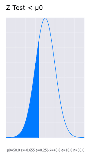
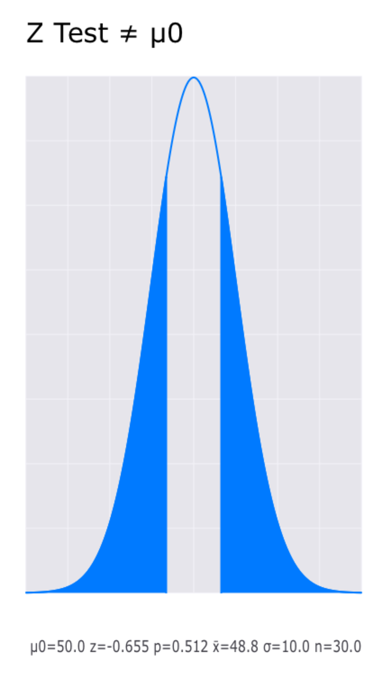
Use the "P<zT(μ0)", "P>zT(μ0)", "P≠zT(μ0)" keys to generate z-Test plots

Value	Keystrokes	Display	Description
50	shift P<zT(μ0)	-0.655	Generates the plot.

Value	Keystrokes	Display	Description
50	shift P≠zT(μ0)	-0.655	Generates the plot.

Use the "z int(cl)" key to calculate z confidence intervals.

Calculate the z confidence interval for the sample data for a standard deviation of 10.
The calculations assume that the sample data has been entered into list x. If this is not the case, the values for the mean and n can be entered instead of calculated.

Value	Keystrokes	Display	Description
	x̄	48.8	Calculates the mean.
10	s	10.0	Stores the standard deviation.
	n	30.0	Calculates n.
.95	z int(cl)	7.16	Calculates the z interval for a 0.95 confidence level and displays the interval.
	ROLL	45.2	Displays the lower value of the interval.
	ROLL	52.4	Displays the upper value of the interval.

Use the "P(<z)", "P(<z)", "P(<z)", "P(<z)" keys to generate PDF plots

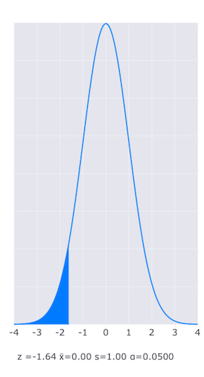
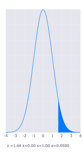
These keys can be used to generate plots of the PDF based on the z, x̄ and s values with the lower tail, upper or both tails shaded.

To plot a lower tail shaded plot of the value of z where the CFD = 0.05:

Value	Keystrokes	Display	Description
0	x̄	0.00	Stores the mean.
1	s	1.00	Stores the standard deviation.
0.05	Φ(z)	0.05	Stores the CDF value.
	z	-1.64	Calculates the zvalue.
	shiftP(<z)	-1.64	Displays the plot.

To plot an upper tail shaded plot of the value of z where the CFD = 0.95:

Value	Keystrokes	Display	Description
0	x̄	0.00	Stores the mean.
1	s	1.00	Stores the standard deviation.
0.95	Φ(z)	0.05	Stores the CDF value.
	z	1.64	Calculates the zvalue.
	shiftP(>z)	1.64	Displays the plot.

To plot a 2 tail shaded plot of the sample data for the value of z =30:

Value	Keystrokes	Display	Description
	x̄	48.8	Calculates the mean.
	s	9.50	Calculates the standard deviation.
30	z	30.0	Stores the z value.
	shift(<z>)		Displays the plot.

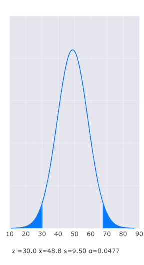
Note that the CDF value has been calculated in order to calculate the α value.

To plot a center shaded plot of the sample data for the value of z =45:

Value	Keystrokes	Display	Description
	x̄	48.8	Calculates the mean.
	s	9.50	Calculates the standard deviation.
45	z	45.0	Stores the z value.
	shift(>z<)		Displays the plot.

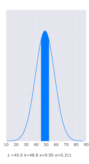
Other shading and plotting options can be achieved by plotting the PDF as an expression, "dnorm(rgx, mean, sd)" using the Expressions Focused Calculator.