Plotting Examples
This page contains examples for the "plot", "plot(n)", "shade p", "exprna=b", "shade[]", and "param" plotting keys from the Expression calculator.
Plot using the "plot" key.
Using the Expressions calculator, use the "plot" key to plot the expression:
.2×rgx^3-2×rgx+6
from rgx = -4 to 4
| Value | Keystrokes | Display | Description |
|---|---|---|---|
| C | Clears the expression. | ||
| .2×rgx^3-2×rgx+6 | Enter the expression to plot. | ||
| K | Enters K mode. | ||
| 4 | STO xMax | 4.00 | Stores the max value the plot. |
| +/- STO xMIN | -4.00 | Stores the min value the plot. | |
| plot | Displays the plot |

Plot Multiple expressions using the "plot(n)" key.
Using the Expressions calculator, use the "plot(n)" key to plot the expressions:
.2×rgx^3-2×rgx+6
.2×rgx^3-3×rgx+6
from rgx = -4 to 4.
| Value | Keystrokes | Display | Description |
|---|---|---|---|
| C | Clears the expression. | ||
| .2×rgx^3-2×rgx+6 | Enter the expression to plot. | ||
| STO exprna | Stores the expression as exprna | ||
| C | Clears the expression. | ||
| .2×rgx^3-3×rgx+6 | Enter the expression to plot. | ||
| STO exprnb | Stores the expression as exprnb | ||
| 4 | STO xMax | 4.00 | Stores the max value the plot. |
| +/- STO xMIN | -4.00 | Stores the min value the plot. | |
| 2 | plot(n) | Displays the plot |
In this example, after entering the first expression and storing it, you can use the expression editor (double tap the expression) to change the 2 to a 3 instead of re-entering the expression.
plot(n) will plot up to 5 expressions stored in exprna - exprne.

Shaded plot using the "shade p" key.
Using the Expressions calculator, use the "shade p" key to plot the expression:
.2×rgx^3-2×rgx+6
from rgx = -4 to 4, with shading from -4 to 0.
| Value | Keystrokes | Display | Description |
|---|---|---|---|
| C | Clears the expression. | ||
| .2×rgx^3-2×rgx+6 | Enter the expression to plot. | ||
| K | Enters K mode. | ||
| 4 | STO xMax | 4.00 | Stores the max value the plot. |
| +/- STO xMIN | -4.00 | Stores the min value the plot. | |
| STO x1 | -4.00 | Stores the x1 value. | |
| 0 |
STO x2 | 0.00 | Stores the x2 value. |
| shade p | Displays the plot |

Shaded plot with multiple shaded areas using the "shade []" key.
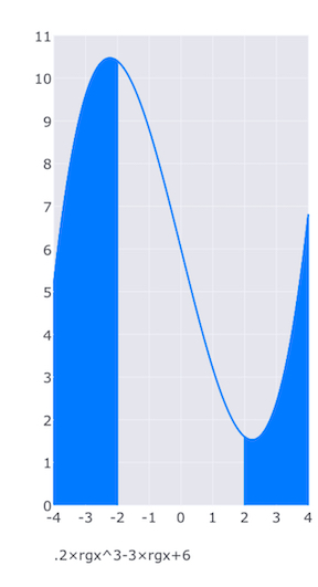
Using the Expressions calculator, use the "shade[]" key to plot the expression:
.2×rgx^3-2×rgx+6
from rgx = -4 to 4, with shading from -4 to -2 and 2 to 4.
"listx"contains the list of the values for the shaded areas. This examples demonstrates 2 shaded areas, but more can be added.
| Value | Keystrokes | Display | Description |
|---|---|---|---|
| C | Clears the expression. | ||
| .2×rgx^3-2×rgx+6 | Enter the expression to plot. | ||
| K | Enters K mode. | ||
| 4 | STO xMax | 4.00 | Stores the max value the plot. |
| +/- STO xMIN | -4.00 | Stores the min value the plot. | |
| Open the List Manager and select list x | |||
| (trash button) |
Clear the list. | ||
| + + + + |
Create 4 rows. | ||
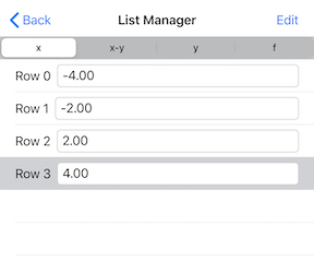
| -4 -2 2 4 |
Enter the values. | ||
| shade[] | Displays the plot |
List Manager with shading values entered:
Parametric Plot using the "param" key.
Using the Expressions calculator, use the "param" key to plot the path of a ball with respect to the time in rgx.
x axis values = rgx×v×cos(a)
y axis values = rgx×v×sin(a)-0.5×g×rgx^2
Where rgx is the time, v = initial velocity, a = the initial angle, g = 9.81 (gravitational acceleration m/sec^2).
v, a and g will be stored so different velocities and angles can be plotted.
| Value | Keystrokes | Display | Description |
|---|---|---|---|
| C | Clears the expression. | ||
| 9.81 |
STO g | 9.81 |
Stores the g value |
| 30 |
STO v | 30.0 |
Stores the v value |
| 25 | STO a | 25.0 | Stores the a value. |
| rgx×v×cos(a) | Enters the x axis expression. | ||
| STO exprna |
Stores the x axis expression. | ||
| rgx×v×sin(a)-0.5×g×rgx^2 | Enters the y axis expression. | ||
| STO exprnb | Stores the y axis expression. | ||
| 0 |
STO xMin |
0.00 |
Stores xMin |
| 2.58 | STO xMax | 2.58 |
Stores xMax |
| shift param | displays the plot. |
RCL v, RCL a, RCL g will enter the v, a, g varaibles, respectively, when entering the expressions.
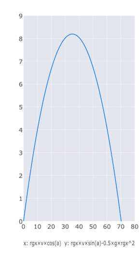
The xMax value of 2.58, when the ball height = 0 was calculated using the "solve(y)" key with the y axis expression.
Different values for variables g, v and a can be entered and plotted.